Anime Recommendation Engine
Motivation
Anime is a form of animated media with origins tied to Japan. A recent Google trend revealed that there are between 10-100M searches for anime related topics every month [1]. This number has only just peaked in recent months as a result of nation-wide quarantine orders and subsequent efforts to find an entertainment medium [2]. Our goal is to apply machine learning to recommend the best anime for a user to watch based on their personal favorites. Recommendation engines can be built using the techniques of either collaborative or content-based filtering. Due to the limitations of our dataset, our implementation involved using content-based filtering with a modified KNN. To enhance the model and provide only the best of recommendations, we used a combination of dense, categorical, and textual features.
Data
Dataset Description
We utilized a dataset that we found through a GitHub project called tidy.csv that had been constructed from cleaning a kaggle dataset [3]. In our complete original dataset, we have 77,911 records with each consisting of 28 features. These features include:
| Name | Description | Type |
|---|---|---|
| animeID | Uniquely identifies each of the 13,631 included animes | dense |
| name | Anime title | categorical |
| title_english | Anime title in English | categorical |
| title_japanese | Anime title in Japanese | categorical |
| title_synonyms | Nicknames or other known names for the anime | categorical |
| type | Anime type such as Movie, Music, ONA, OVA, Special, TV, or Unknown | categorical |
| source | Anime source such as Original, Manga, Book, Game, Music, etc. (16 unique) | categorical |
| producers | Producer of the anime (1,073 unique) | categorical |
| genre | Anime genre such as Action, Sci-Fi, Fantasy, etc. (40 unique) | categorical |
| studio | The studio creating the anime (47 unique) | categorical |
| episodes | The number of episodes in the anime (range from 1 to 3,057) | dense |
| status | Status of “Currently Airing” or “Finished Airing” | categorical |
| airing | TRUE if Status is “Currently Airing”, FALSE otherwise | categorical |
| start_date | Date that the anime started airing (ranges from 1/1/1917 to 2/3/2019) formatted as ymd | categorical |
| end_date | Date that the anime stopped airing (ranges from 2/2/1962 to 9/2/2019) formatted as ymd | categorical |
| duration | Episode length such as 24 min, 1 hr 55 min, etc. (ranges from 7 sec to 3 hr 51 min) | categorical |
| rating | Audience rating such as None, G, PG, PG-13, R 17+, or R+ | categorical |
| score | Average rating for the anime (ranges from 1 to 10) | dense |
| scored_by | Number of people who scored the anime (ranges from 0 to 1,107,955) | dense |
| rank | Rank of the anime (ranges from 1 to 13,838) | dense |
| popularity | Popularity rank according to MyAnimeList.net (ranges from 1 to 15,474) | dense |
| members | Number of community members in the anime’s group (ranges from 6 to 1,610,561) | dense |
| favorites | Number of times the anime has been added to a person’s favorites (ranges from 0 to 120,331) | dense |
| synopsis | Paragraph description of the anime storyline | textual |
| background | Paragraph description of the history behind the anime’s creation | textual |
| premiered | Season that the anime premiered (ranges from Spring 1961 to Winter 2019) | categorical |
| broadcast | Scheduled broadcast time each week for the anime | categorical |
| related | Any known related anime series | categorical |
Figure 1: Anime Count Comparisons by Type and Source
Figure 2: Anime Count Comparison by Genre and Airing Status
Figure 3: Anime Count Comparisons by Rating and Score
Figure 4: Average Score of Most Reviewed Producers and Studios
Figure 5: Anime Count by Decade of Premier
Pre-processing
Before we were able to use the data, we first had to clean it by removing the unnecessary columns and replacing NA values with 0s. Although our dataset had 77,911 rows, many of these rows were duplicated multiple times for a single anime title. For example, the anime Cowboy Bebop was duplicated 17 times, once for each genre, each studio, and/or each producer that worked on the anime. To clean this up, we grouped all the anime together by title, and consolidated the information to remove the duplicated rows - ultimately condensing our dataset from 77,911 rows to 2,856 unique anime. Following this, we also one-hot encoded all of the categorical data columns (i.e. genre, studio, source, producers, rating, type). One-hot encoding not only reduced the number of rows in our dataset by ensuring that each anime only occupied one row, but also prepared the dataset for constructing the vectors during the data modelling phase.
In addition to the categorical data columns, our dataset conveniently held a wealth of information for us in the form of a textual synopsis for each anime. To utilize of this, we used a pretrained word2vec model by Google that was trained on the Google News corpus (over 300 billion words) to output 300-dimensional word vectors. The idea was to use the word embeddings to capture the semantics of the summary in an attempt to use these features to find other anime with similar summaries in semantics. In order to ensure that the input to the model was standardized, the synopsis for each anime was pre-processed to ensure that they were properly formatted and consisted of only words of interest. We removed all punctuations and capitalization, as well as common words such as “a”, “an”, and “in” using the list of default stopwords used by MySQL’s MyISAM search indexes [4]. This significantly reduced the amount of words we were working with as the size of our word bank decreased from 34354 to 21259, and the maximum length of the synopses decreased from 540 to 290. We then computed a 1x300 synopsis summary vector for each anime by plugging in every word of the synopsis into the word2vec model and averaging all of the vectors. Note, fictional words specific to an anime (such as “Geass” or names like “Lelouch”) may not generate a resulting word embedding, in which case the word is simply ignored in the final calculation of the synopsis summary vector.

Figure 6: Synopsis summary vector
Ultimately, each anime had a corresponding feature vector of shape 1x414. To better understand our feature set and intrinsic relationships amongst features, the following correlation matrices (performed on subsets of features for visibility) were generated:
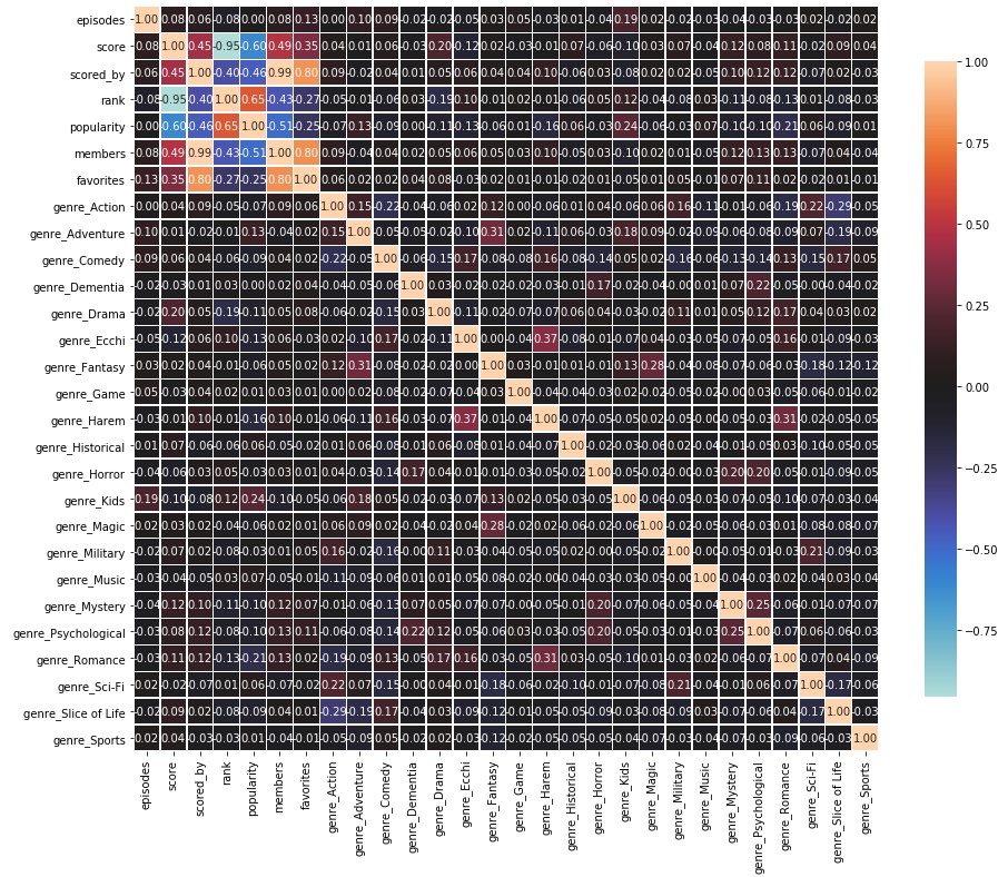
Figure 7: Correlation matrix for stats and genre features
The above stats correlation matrix shows many expected behaviors. For example: a very strong negative correlation between score and ranking, and a very strong positive correlation between members and number of favorites. Likewise, there are relatively strong positive correlations between the genres of “Ecchi” and “Harem”, and “Fantasy” and “Magic”. Particularly interesting was the fact that anime with the genre “Kids” had a much higher chance of being popular while anime labelled as “Romance” were more likely to be less popular.
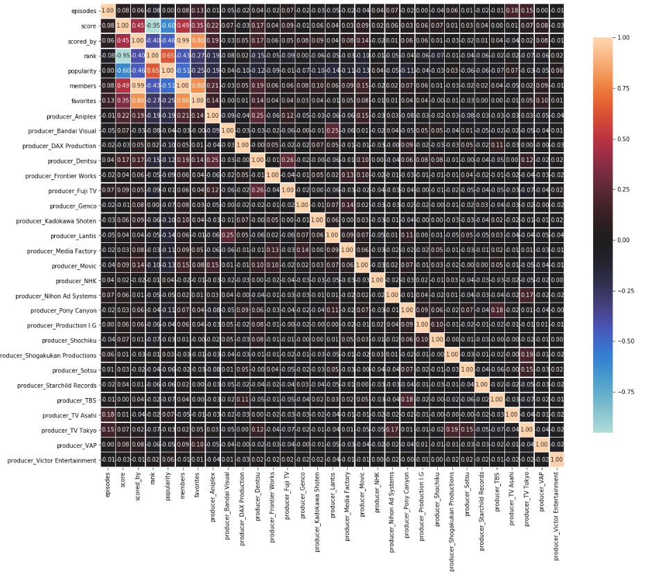
Figure 8: Correlation matrix for stats and producer features
The above correlation matrix shows the correlation matrix for the subset of our features containing information on the producer. While there were many producers to consider, the more notable ones: Aniplex, a flagship animation company owned by Sony, and Dentsu, Japan’s largest advertising company, had positive correlations with respect to their scores, number of favorites, and number of members.
PCA
Due to the fact that our feature space was so large (primarily as a result of using textual features), we attempted to reduce the feature space by using PCA. By graphing the summed captured variance of each component, we deduced that using 300 components out of the total 412 was suitable for our needs as it covered 98% of the variance of our feature set. This PCA’ed version of our feature set was then used in our KNN model to find the best anime recommendations.
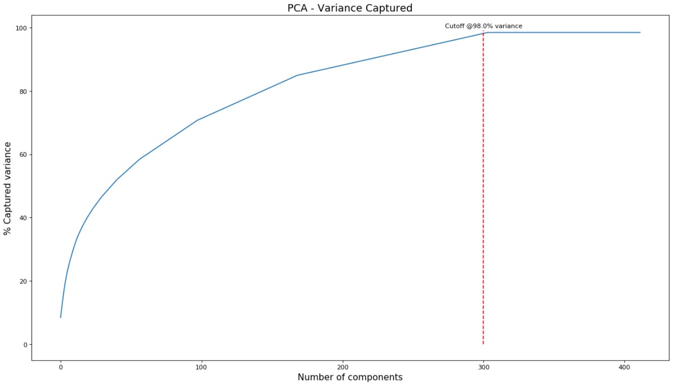
Figure 9: Captured variance of 300 components was 98%
In an attempt to better visualize the feature space, and the relative space and groupings of anime, we used PCA to convert down to 2D space. It is important to note that using 2 features only captures 12.2% of the total variance in our feature set, and thus the feature space visualization is not optimal but merely serves as a visualization to gain a better understanding of the dataset.
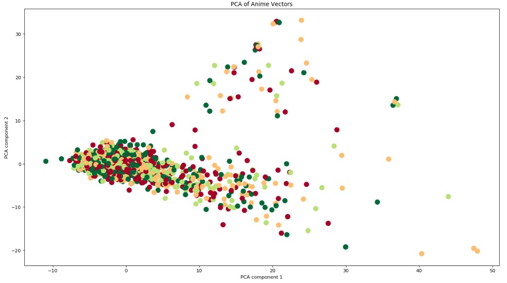
Figure 10: PCA of feature space into 2D space
DBSCAN
The PCA graph in 2 dimensional space showed clearly distinct clusters of anime which made us wonder exactly how these clusters formed and what type of anime were represented in each cluster. To tackle this problem, we converted our feature space to 300 dimensions (same feature space as our input to KNN), and performed DBSCAN, an unsupervised clustering algorithm. In order to properly use DBSCAN, we tuned the minpts parameter by hand such that not all the points were located in one cluster nor were there an exceptionally large number of noise points. Note, we could not use the heuristic of minpts <= D+1, because D would have been set to ~301 or ~13% of our entire dataset. We set minpts=3. Epsilon was tuned by graphing and sorting the distances of the 10th nearest neighbor of each point in 300 dimensional space. The “elbow method” was used to set epsilon to 30.
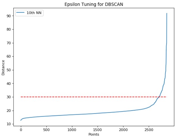
Figure 11: Elbow method to tune the epsilon parameter for DBSCAN
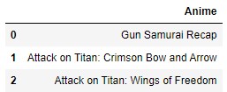
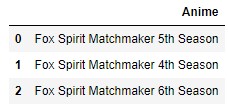
The resulting DBSCAN consisted of 4 clusters and 97 noise points. Below is a representation in 2D space.
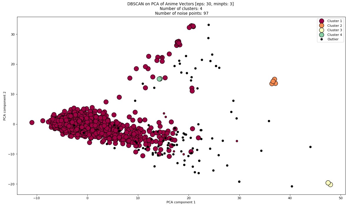
Figure 12: DBSCAN on PCA of feature space
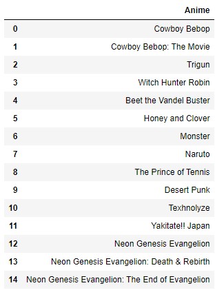
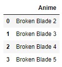
Below is a deeper dive into a subset of specific anime within each cluster:
| Cluster 1 | Cluster 2 | Cluster 3 | Cluster 4 | Cluster Outlier |
|---|---|---|---|---|
 |
 |
 |
 |
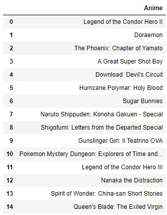 |
Figure 13: Top-15 anime represented in each cluster
Modelling & Results
Modelling
The KNN algorithm seeks to find the k most similar anime to the current anime. However, often times it is very difficult for users to be able to capture the full breadth of their anime preferences in a single anime. In our modified KNN algorithm, we allow users to input an arbitrary amount of anime that they like in an attempt to better understand and recommend anime catered to their preference. Assume a user inputs n different anime that they enjoyed. To model this, we average out the n feature vectors of each of those anime and compute KNN on this new vector that ideally captures the essence of each of their preferred animes.

Figure 14: KNN input vector
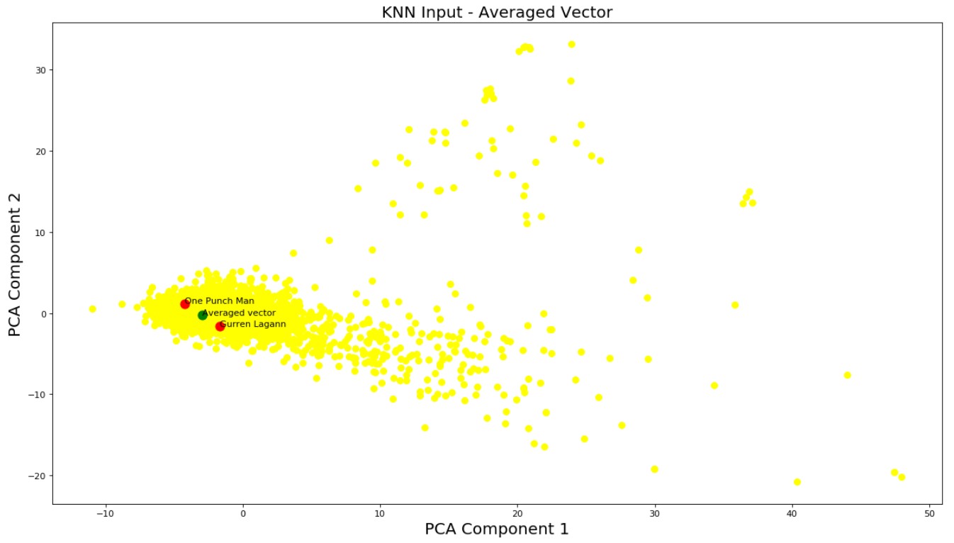
Figure 15: Graphical representation of KNN input vector
There were two distance metrics that we considered for our modelling. The first, and preferred method, was using cosine similarity. Cosine distance is defined as:
and measures the angle between our input average feature vector and each of the feature vectors for anime in the dataset. We preferred cosine similarity as a distance measurement due to the way our dataset values were distributed. To process our data, we one-hot encoded our categorical data values, like genre, studio, and source. These columns were represented in our processed data in 1s and 0s. In comparison, our originally quantitative feature data values, such as episodes, which had values ranging from 1 to 1787, and scored_by, with minimum at 8 and maximum value 1107995, were much greater than our one-hot encoded values, and could possibly skew our KNN results towards the originally quantitative features. With this in mind, we implemented Cosine similarity as a distance measurement because it focuses on the angle between the vectors, and does not consider the respective weights or magnitudes of the vectors.
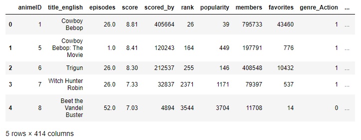
Figure 16: Anime Dataset example data, genre_Action (far right) is an example of one-hot encoding of categorical feature genre
Our alternative distance metric was using Euclidean distance, measured by:
Euclidean distance, in contrast to Cosine distance, is similar to measuring the actual distance between the two vectors, and is thus affected by angle and magnitude of the vectors. We implemented Euclidean distance as an alternative distance measurement because we were interested in seeing how the different distance functions would perform comparatively to each other.
For our KNN implementation, we compare the distance values of each feature vector to our input average vector. When considering Euclidean distance, this can be compared directly (ex. d(x1,average) = 7.8 < 12 = d(x2,average)). However, the same does not apply for Cosine similarity. A Cosine similarity value (CosTheta) of 0 actually corresponds to an angle of 90 degrees, while a Cosine similarity of 1 corresponds with 0, so they cannot be compared as is. Specifically, we have to shift our Cosine similarity such that a low Cosine distance value corresponds with a low angle. We chose to implement this by representing Cosine distance as:
which then ensures minimum angle, 0 degrees, is represented as 1-Cos(0) and thus a minimum Cosine distance value of 0 as well. In contrast, now for an angle of 90 degrees, Cosine distance = 1-Cos(90) = 1-Cos(-90) = 1, and for an angle of 180 degrees, Cosine distance = 1-Cos(180) = 2, the maximum Cosine distance value.
Results
Because we are using an unsupervised learning model, there is no sure-fire way to measure the “accuracy” of our results. However, we came up with several comparitive statistical measurements to analyze our recommendations relative to our inputs.
The first measurement we use is the standardized average distance between the average of the input feature vectors and the feature vector for the anime in question, which we refer to as STD Distance. STD Distance takes its derivation from standard deviation and is calculated by:
where for all xi in the set of result anime feature vectors, n is the number of recommended animes, and u is the average feature vector generated from the input animes. It essentially represents the average variance of the set of recommended anime features from the input average features.
Another metric that we use to compare our overall recommendations to our input animes is average distance:
and is simply the mean value of all the distances of our output anime.
For our feature comparisons, we defined two major measurements. The first is Average Absolute Standard Z-score of the feature of the output anime. Standard Z-score of anime i refers to the standardized difference of the value of the anime feature from the mean input feature value and is defined by:
where xf is the value of feature f in anime feature vector x, mu is the average value for that feature from our input animes, and sigma is the standard deviation of that feature from all our of data values. From Standard Z-score, we define Average Absolute Standard Z as:
Our second primary metric for feature comparisons is Average Standard Feature Deviation, derived similarly to standard deviation:
where fi is the feature value of the output anime, mu is the average value for that feature from our input animes, and n is the number of output anime.
EXAMPLE 1: From a single anime
[‘Attack on Titan’]
We first chose a single anime to test our KNN model with. This represents an input set with fully minimized variability. Recommendations are as follows:
| Cosine Unaltered | Cosine Normalized | Euclidean Unaltered | Euclidean Normalized | |
|---|---|---|---|---|
| STD Input Distance | 1.11e-16 | 2.22e-16 | 0 | 0 |
| Distances | - Sword Art Online: 4.53e-05 - Dragon Ball Z: 4.82e-05 - Code Geass: Lelouch R2: 5.28e-05 - Death Note: 5.83e-05 - One Punch Man: 1.59e-04 |
- Attack on Titan S2: 0.26 - Fullmetal Alchemist: Brotherhood: 0.36 - Death Note: 0.38 - Code Geass: Lelouch: 0.40 - Code Geass: Lelouch R2: 0.44 |
- Sword Art Online: 68802.63 - Death Note: 132434.60 - Fullmetal Alchemist: Brotherhood: 261364.26 - One Punch Man: 384929.08 - Tokyo Ghoul: 459418.36 |
- Attack on Titan S2: 17.51 - Code Geass: Lelouch: 21.16 - Code Geass: Lelouch R2: 21.60 - Fullmetal Alchemist: Brotherhood: 22.11 - Akame ga Kill: 22.31 |
| AVG Distances | 7.29e-05 | 0.37 | 261389.78 | 20.94 |
Quantitative Feature Comparisons from EXAMPLE 1
popularity (Mean: 2988.34, St. Dev: 2868.05)
| Distance | Normalized | Avg Abs St. Z | Avg Sq St. Dev |
|---|---|---|---|
| Cosine | no | 0.01 | 32.42 |
| Cosine | yes | 0.01 | 20.45 |
From the above table for popularity feature standard deviation, we can see that the popularity values of Cosine un-normalized KNN results are on average further from the input average of the popularity feature compared to the Cosine normalized KNN. This is directly opposite from our feature analysis of scored_by results. However, it should be the popularity of an anime is inversely proportional to its value for the popularity feature. For example, an anime with popularity feature value 4 is mmore popular than an anime with popularity feature value 200. It is likely Cosine normalized KNN performed better than Cosine un-normalized KNN for the popularity feature as our input anime had a popularity of 2, which is a small value and is likely less skewed when normalized.
members (Mean: 100507.59, St. Dev: 164257.15)
| Distance | Normalized | Avg Abs St. Z | Avg Sq St. Dev |
|---|---|---|---|
| Cosine | no | 2.45 | 516539.41 |
| Cosine | yes | 2.47 | 474466.31 |
From the above table for members feature standard deviation, we can see that the members values of Cosine normalized KNN results are on average further from the input average of the members compared to the Cosine un-normalized KNN. This is likely because our input members value was 1500958, a high value that may have been skewed by normalization as the members feature also has a high range (52 to 1610561).
favorites (Mean: 1610.34, St. Dev: 6211.04)
| Distance | Normalized | Avg Abs St. Z | Avg Sq St. Dev |
|---|---|---|---|
| Cosine | no | 4.75 | 31280.51 |
| Cosine | yes | 5.22 | 38706.69 |
The results for the favorites feature was similar to that of the members feature. Like members, the favorites feature has a large range (0 to 120331) and our input anime had a high favorites value of 70555 (3rd quartile).
If we compare Average Absolute Standard Z between our quantitative features, favorites had the largest average absolute standard Z. We can expect this, because the favorites feature has a large range of values (from 0 to 120331) and a moderately high variance (6211.04) for its range. Of the features, popularity had the lowest average absolute standard z. Although the range of feature popularity is relatively large (from 1 to 15013), the data distribution for popularity is right-skewed:

and the bulk of the data for popularity is small in value. Because of this distribution, we were able to get results with small variance based on our input popularity, 2. In contrast, if we were to run KNN for an input with larger popularity feature, we would get significantly different results (see below).
Partial feature test, Median popularity input (Mean: 2988.34, St. Dev: 2868.05)
| Distance | Normalized | Avg Abs St. Z | Avg Sq St. Dev |
|---|---|---|---|
| Cosine | no | 0.05 | 180.49 |
Our resulting average absolute standard Z for our popularity feature from this test is 0.05, which is much greater than our EXAMPLE 1 test results (average absolute standard Z: 0.01).
EXAMPLE 2: From a single series of anime
[‘Attack on Titan’, ‘Attack on Titan: Since That Day’, ‘Attack on Titan: Crimson Bow and Arrow’, ‘Attack on Titan: Wings of Freedom’, ‘Attack on Titan Season 2’, ‘Attack on Titan: Junior High’, ‘Attack on Titan Season 3’]
For this KNN test, we selected a series of anime to represent a very closely associated anime input set. We ran our KNN model and received the following results:
| Cosine Unaltered | Cosine Normalized | Euclidean Unaltered | Euclidean Normalized | |
|---|---|---|---|---|
| STD Input Distance | 1.11e-16 | 2.22e-16 | 0 | 0 |
| Distances | - anohana: 9.24e-06 - Madoka Magica the Movie: 1.40e-05 - Kuroko’s Basketball 1.42e-05 - Vampire Knight: 2.51e-05 - Maid Sama!: 2.68e-05 |
- Gun Samurai Recap: 0.12 - Marches Comes in Like a Lion: 0.18 - Berserk: Recollections: 0.24 - So, I Can’t Play H!: 0.26 - Tsukigakirei: First Half: 0.31 |
- Miss Kobayashi’s Dragon Maid: 10003.85 - Rosario + Vampire: 10933.50 - My Teen Romantic Comedy: 13918.15 - GATE: 16494.10 - JoJo’s Bizarre Adventure: 18196.80 |
- Marches Comes in Like a Lion: 21.31 - Persona 4 the Animation: 27.07 - Fullmetal Alchemist: Premium: 29.63 - Shiki Specials: 29.80 - Robot Girls Z: 30.68 |
| AVG Distances | 1.79e-05 | 0.23 | 13909.29 | 27.70 |
Quantitative Feature Comparisons from EXAMPLE 2
members (Mean: 100507.59, St. Dev: 164257.15)
| Distance | Normalized | Avg Abs St. Z | Avg Sq St. Dev |
|---|---|---|---|
| Cosine | no | 1.03 | 192446.07 |
| Cosine | yes | 2.21 | 376356.68 |
| Euclidean | yes | 2.38 | 391837.88 |
| Euclidean | no | 0.50 | 172492 |
For members, both un-normalized KNN had improved average absolute standard Z values (lower), opposed to the normalized average absolute standard Z scores.
favorites (Mean: 1610.34, St. Dev: 6211.04)
| Distance | Normalized | Avg Abs St. Z | Avg Sq St. Dev |
|---|---|---|---|
| Cosine | no | 0.94 | 6467.43 |
| Cosine | yes | 1.90 | 11806.14 |
| Euclidean | yes | 1.92 | 11906.55 |
| Euclidean | no | 1.08 | 7654.53 |
Like our results for the members feature comparison test, un-normalized KNN performed better with regards to the favorites feature as well. However, unlike for members, Cosine un-normalized KNN produced the smallest average absolute standard Z score.
One-Hot Feature Comparisons from EXAMPLE 2
For this series of comparisons, the mean value for one-hot feature represents the percentage of the data that has this feature. Some features have relatively high proportions, such as genre_Comedy, which has a mean value of 0.45 (or 44.86% of the data). In comparison, other features represent a very small percentage of the data, such as studio_Madhouse, which has a mean of 0.05, representing a 5.49% of the data. Additionally, we use Absolute average difference as a measure test how similar our results were to the input. It is calculated by:
where x-bar is the average feature value from the anime recommendations and mu is the average feature value from the inputs.
genre_Action (Mean: 0.40, St. Dev: 0.49)
| Distance | Normalized | Avg Abs St. Z | Avg Sq St. Dev | Abs Avg Diff |
|---|---|---|---|---|
| Cosine | no | 1.75 | 0.86 | 0.86 |
| Cosine | yes | 1.46 | 0.77 | 0.66 |
| Euclidean | yes | 1.75 | 0.86 | 0.86 |
| Euclidean | no | 1.46 | 0.77 | 0.66 |
On average, the tests were about evenly distributed, with Cosine normalized and Euclidean un-normalized performing slightly better than the other two tests. However, as our inputs formed a concentrated set with with moderate variance, so we expect some randomness in our test results.
studio_Madhouse (Mean: 0.05, St. Dev: 0.23)
| Distance | Normalized | Avg Abs St. Z | Avg Sq St. Dev | Abs Avg Diff |
|---|---|---|---|---|
| Cosine | no | 0 | 0 | 0 |
| Cosine | yes | 0 | 0 | 0 |
| Euclidean | yes | 0 | 0 | 0 |
| Euclidean | no | 0 | 0 | 0 |
From our resulting variance measurements, we can see that for one-hot features with very low population represention (small probability), we cannot expect good measurements for how well our recommendations did relative to the input, as most possible data animes fall outside this tiny portion of our data. This is especially exemplified by our measurements from studio_Madhouse values for average absolute standard Z and average standard feature deviation; several times, the values were both 0. However, this value cannot necessarily signify perfect recommendation results for this feature, given the input anime. Instead, this measurement tells us that from our anime dataset, we do not have enough values in our anime dataset to accurately measure our KNN performance with regards to the feature in question. However, with regards to our results, we can say with relative confidence that because we had a set of input anime with a mean studio_Madhouse feature value of 0 (meaning, none of the animes were created by studio_Madhouse) we would expect for our recommendations to return non-studio_Madhouse’s animes.
As with the feature comparison trends, overall Cosine un-normalized KNN results prioritized high valued quatitative features over small value features such as one-hot encoded features. In contrast, Cosine normalized KNN produced results that were heavily impacted by one-hot encoded data values like our synopsis encoded data. Seen below is an excerpt of our input synopses:

which heavily featured words like “recap” and “episode.” Interestingly, our resulting recommendations from Cosine normalized KNN also produced recommended animes based on these wordings (see below).

Similarly, our Euclidean normalized KNN results also were heavily based on our synopsis key wordings (as seen below):

In contrast, our Euclidean un-normalized results were heavily based on high values quantitative features such as members, and did not give results similar to our on-hot encoded features. We can conclude from these results that normalizing our data is imperative to giving equal emphasis to our one-hot features and quantitative data features, but may result in skew due to normalizing high value quantitative feature values.
EXAMPLE 3: From a relatively similar assortment of anime
[‘Attack on Titan’, ‘Attack on Titan Season 2’, ‘Bungo Stray Dogs’, ‘My Hero Academia 3’, ‘Nanbaka’, ‘Nanbaka: Season 2’, ‘Nanbaka: Idiots with Student Numbers!’, ‘One Punch Man’]
Using our personal anime knowledge and experiences, we selected a set of anime that were relatively closely associated for our KNN model testing. Below are our KNN model recommendations:
| Cosine Unaltered | Cosine Normalized | Euclidean Unaltered | Euclidean Normalized | |
|---|---|---|---|---|
| STD Input Distance | 1.73 e-03 | 0.29 | 1149911.69 | 20.27 |
| Distances | -Fullmetal Alchemist: 7.40e-06 -Future Diary: 9.45e-06 -Elfen Lied: 9.74e-06 -Parasyte: 2.14 e-05 -My Teen Romantic Comedy: 2.59e-05 |
-Fullmetal Alchemist: Brotherhood: 0.50 -My Hero Academia: 0.51 -Code Geass: Lelouch: 0.52 -Death Note: 0.52 -Code Geass: Lelouch R2: 0.52 |
-Ouran High School Host Club: 8961.68 -Maid-Sama!: 13454.21 -My Teen Romantic Comedy: 15365.79 -Princess Mononoke: 18975.94 -Overlord: 19197.70 |
-JoJo’s Bizarre Adventures: Diamond is Unbreakable: 12.12 -Re:CREATORS: 12.39 -Akame ga Kill!: 12.40 -Drifters: 12.47 -JoJo’s Bizarre Adventure: Stardust Crusaders: 12.76 |
| AVG Distances | 1.47e-05 | 0.52 | 15191.06 | 12.43 |
One-Hot Feature Comparisons from EXAMPLE 3
genre_Comedy (Mean: 0.45, St. Dev: 0.50)
| Distance | Normalized | Avg Abs St. Z | Avg Sq St. Dev | Abs Avg Diff |
|---|---|---|---|---|
| Cosine | no | 1.11 | 0.60 | 0.35 |
| Cosine | yes | 1.11 | 602 | 0.35 |
| Euclidean | yes | 1.11 | 0.60 | 0.35 |
| Euclidean | no | 0.90 | 0.51 | 0.15 |
From the above feature comparison, we can see that of the KNN tests, Euclidean un-normalized had the worst performance. This most likely because of how the Euclidean formula is defined to consider weights and magnitudes of the vectors in comparison and, because the test was also not normalized, the final outcome was biased towards largest quantitative features, such as members, or favorites (which we can see from the previous favorites and members feature comparison tables that Euclidean un-normalized had the highest accuracy for, out of all our KNN tests).
EXAMPLE 4: From different anime genres
[‘AKIRA’, ‘Desert Punk’, ‘Naruto’, ‘D.N.Angel’, ‘Rurouni Kenshin’]
We selected our animes in this test by choosing 5 random genres (Horror, Ecchi, Comedy, Magic, and Romance) and then choosing an anime from the top of the list of anime in the corresponding genre. We then put this set of anime into our KNN model. The results were as follows:
| Cosine Unaltered | Cosine Normalized | Euclidean Unaltered | Euclidean Normalized | |
|---|---|---|---|---|
| STD Input Distance | 8.94e-05 | 0.54 | 50161.62 | 12.04 |
| Distances | -anohana: 1.02-05 -Parasyte: 1.36e-05 -Elfen Lied: 1.36e-05 -Future Diary: 2.93e-05 -Vampire Knight: 3.67e-05 |
-Naruto: Shippuden: 0.51 -Bleach: 0.53 -Dragonball Z: 0.54 -Tokyo Ghoul √A: 0.59 -Reborn!: 0.59 |
-Haikyu! 2: 6305.24 -Nisemonogatari: 10319.20 -School Days: 12258.90 -Wolf Children: 12704.43 -Kuroko’s Basketball 2: 12971.85 |
-JoJo’s Bizzare Adventure: Stardust Crusaders: 11.15 -Drifters: 11.24 -Jojo’s Bizarre Adventure: 11.54 -Evangelion 3.0: 11.63 -Re:CREATORS: 11.68 |
| AVG Distances | 2.38e-05 | 0.55 | 10911.93 | 11.45 |
One-Hot Feature Comparisons from EXAMPLE 4
genre_Drama (Mean: 0.27, St. Dev: 0.44)
| Distance | Normalized | Avg Abs St. Z | Avg Sq St. Dev | Abs Avg Diff |
|---|---|---|---|---|
| Cosine | no | 1.81 | 0.89 | 0.80 |
| Cosine | yes | 0.45 | 0.45 | 0.20 |
| Euclidean | yes | 0.91 | 0.63 | 0.40 |
| Euclidean | no | 0.91 | 0.63 | 0.40 |
From the genre_Drama feature table above, we can see that Cosine normalized performed the best, with a lowest absolute average difference of 0.2, while Cosine un-normalized had the worst performance, with absolute average difference of 0.80.
Comparative Quantitative Feature Comparisons, EXAMPLE 3 and 4
| EXAMPLE 3 (similar inputs) | EXAMPLE 4 (different inputs) | |||
|---|---|---|---|---|
| Distance | Normalized | Avg Abs St. Z | Avg Abs St. Z | |
| members | Cosine | no | 1.76 | 2.33 |
| Cosine | yes | 3.63 | 1.96 | |
| Euclidean | yes | 1.91 | 0.03 | |
| Euclidean | no | 0.04 | 1.15 | |
| favorites | Cosine | no | 0.87 | 1.45 |
| Cosine | yes | 9.01 | 2.81 | |
| Euclidean | yes | 1.46 | 1.03 | |
| Euclidean | no | 0.07 | 1.44 |
From the above table, we can see that for a similar set (Example 3), both un-normalized KNN tests perform more accurately for large quantitative features. From the Example 4 results, we can see that regardless of input set variability, Cosine normalized performs the badly for large quatitative features, which we expect as it both disregards magnitude and weight of vectors (Cosine distance) and has been rebalanced (normalization) so that quantitative features and one-hot features are weighted more evenly. Note that we cannot decisively conclude from our Example 4 results that un-normalized KNN tests always perform more accurately for large quantitative features. However, the results from Example 4 may be possibly affected by variabilty of input animes.
Comparative One-Hot Feature Comparisons, EXAMPLE 3 and 4
| EXAMPLE 3 (similar inputs) | EXAMPLE 4 (different inputs) | |||||
|---|---|---|---|---|---|---|
| Distance | Normalized | Avg Abs St. Z | Abs Avg Diff | Avg Sq St. Dev | Abs Avg Diff | |
| genre_Comedy | Cosine | no | 1.11 | 0.35 | 1.61 | 0.80 |
| Cosine | yes | 1.11 | 0.35 | 0.64 | 0 | |
| Euclidean | yes | 1.11 | 0.35 | 0.88 | 0.20 | |
| Euclidean | no | 0.90 | 0.15 | 1.37 | 0.60 |
From the above one-hot comparison, we can see that Cosine normalized performs better given more input variability. This can be tied back to our Example 2 results; the translated text encoded values were concentrated around specific words (specifically “recap” and “episode”) and the resulting anime recommendations were skewed toward animes with similar text synopses, rather than even coverage of all one-hot and quantitative features. In contrast, when there is more input variability, there is less chance to bias the Cosine normalized output to a specific encoded feature. For a similar set of inputs, we can see that Euclidean un-normalized performs slightly better than the other tests. However, we cannot definitively say whether this is due to randomness or not. Additionally, we can identify that for both similar anime sets and different anime sets Cosine un-normalized performed the worst for one-hot encoded features.
Overall Analysis
From our results, we can see for our dataset that on average, Euclidean un-normalized KNN preformed the weakest (highest average output distance). This is likely due to the range of values we have in our dataset. We processed our categorical data into one-hot encoding, as well as retained quantitative values. In comparison, the range and variation of the quantitative values are very high. For example, quatitative feature scored_by has a range from 8 to 1107955, mean of 51396.65, and a standard deviation of 96648.63. Without normalization, using Euclidean distance, which accounts for weight of vectors, as well as the angle between them, will be skewed toward higher values, such as scored_by. In contrast, Cosine un-normalized KNN did a better job for considering quantiative data features.
However, to properly take in our NLP one-hot encoded synopsis data, we should use normalized KNN for better results. This accuracy is improved when a set input anime have closely overlapping or related words. For instance, from our Example 3 Cosine normalized KNN test, the input anime synopses shared words like “human”, “hero”, “villain”, “criminal”, “fight”, and “school”. In comparison, the corresponding anime recommendations featured words also featured related words, such as “human”, “killer”, “hero”, “school”, “criminal”, “vigilante”. However, this also has its own downfalls, as quantitative values and one-hot encodes data are normalized to even their weights, more recommendations become heavily dependent on one-hot data. For example, in EXAMPLE 2, specifically the Cosine normalized KNN test, the input anime series (Attack on Titan) had many unrelated but repeating words, such as “recap”, “rewrite”, “episode”, “humanity” and especially contained the phrase “recap of episodes”. Likewise, the synopses of the output animes contained this phrase “recap of episode” or a similar variant, but the recommendations were more dependent on this particular synopsis wording, rather than other features. In contrast, Cosine un-normalized consistently performed the worst for one-hot encoded features.
Additionally, we found that for very different input animes, like in our Example 4 test, the KNN recommendations would have higher variance on average, with normalized KNN results having higher variance than un-normalized KNN.
Conclusion
Though this approach yielded interesting results, there are some aspects that could be improved. For instance, our current dataset separates out different animes within the same series. Therefore, it could recommend a user who inputs an anime in the series, another anime within the same series. This is obviously not an ideal outcome because avid anime watchers likely would not be getting anything meaningful out of the recommendation engine. Rather, we want to be able to introduce people to new anime that they otherwise might not have known of. One way to address this issue is to compress all of the animes in a series down to one row which would completely eliminate the possibility of these types of results. We could also introduce random noise or uncertainty, not only to mitigate this problem but also so that the results are more likely to be new and interesting to the users.
References
[1] Ellis, Theo J. “How the Anime Industry Has Grown Since 2004, According to Google Trends.” Anime Motivation, animemotivation.com, 23 June 2018, https://animemotivation.com/anime-industry-growth-2004-to-2018/.
[2] Ellis, Theo J. “Why The Coronavirus Has Made Anime More Popular Than Ever.” Anime Motivation, animemotivation.com, 24 March 2020, https://animemotivation.com/coronavirus-has-made-anime-more-popular/.
[3] Mock, Thomas. “Anime Dataset.” GitHub, GitHub, Inc., 22 April 2019, https://github.com/rfordatascience/tidytuesday/tree/master/data/2019/2019-04-23.
[4] “Full-Text Stopwords.” MySQL, Oracle Corporation, https://dev.mysql.com/doc/refman/8.0/en/fulltext-stopwords.html.